K-NeighborsRegressor 단점에 대해서 알아보자 1) 영역에서 벗어날 경우, 어떻게 되는지?
- 50Cm 일 경우, 예측하는 데 실패가 발생한 이유.In [1]:
import numpy as np
## 데이터 불러오기 및 array 생성.
perch_length = np.array([8.4, 13.7, 15.0, 16.2, 17.4, 18.0, 18.7, 19.0, 19.6, 20.0, 21.0,
21.0, 21.0, 21.3, 22.0, 22.0, 22.0, 22.0, 22.0, 22.5, 22.5, 22.7,
23.0, 23.5, 24.0, 24.0, 24.6, 25.0, 25.6, 26.5, 27.3, 27.5, 27.5,
27.5, 28.0, 28.7, 30.0, 32.8, 34.5, 35.0, 36.5, 36.0, 37.0, 37.0,
39.0, 39.0, 39.0, 40.0, 40.0, 40.0, 40.0, 42.0, 43.0, 43.0, 43.5,
44.0])
perch_weight = np.array([5.9, 32.0, 40.0, 51.5, 70.0, 100.0, 78.0, 80.0, 85.0, 85.0, 110.0,
115.0, 125.0, 130.0, 120.0, 120.0, 130.0, 135.0, 110.0, 130.0,
150.0, 145.0, 150.0, 170.0, 225.0, 145.0, 188.0, 180.0, 197.0,
218.0, 300.0, 260.0, 265.0, 250.0, 250.0, 300.0, 320.0, 514.0,
556.0, 840.0, 685.0, 700.0, 700.0, 690.0, 900.0, 650.0, 820.0,
850.0, 900.0, 1015.0, 820.0, 1100.0, 1000.0, 1100.0, 1000.0,
1000.0])
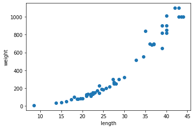
import matplotlib.pyplot as plt
plt.scatter(perch_length, perch_weight)
plt.xlabel('length')
plt.ylabel('weight')
plt.show()
데이터를 훈련세트와 테스트세트로 구분하자. 1) input 데이터는 2차원 for sklearn training을 위해서
In [2]:
from sklearn.model_selection import train_test_split

## 훈련데이터와 테스트데이터 구분하기
train_input, test_input, train_target, test_target = train_test_split(perch_length, perch_weight, random_state=42)

## sklearn.training을 위해서 차원 변경(1차원 --> 2차원)
train_input = train_input.reshape(-1, 1)
test_input = test_input.reshape(-1, 1)

## 최근접 이웃 개수가 3일 경우, modeling training.
from sklearn.neighbors import KNeighborsRegressor

knr = KNeighborsRegressor(n_neighbors=3)

## K-최근접 이웃 회귀 모델 훈련
knr.fit(train_input, train_target)

## 50Cm인 경우, evaluate 하기
print(knr.predict([[50]]))
[1033.33333333]
Investigation for estimation data
In [3]:
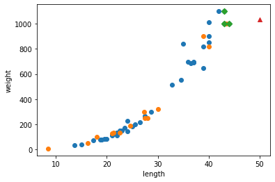
## 해당 데이터의 예측하기 위한 길이와 인덱스가 어떤 데이터인지 확인.
distances, indexs = knr.kneighbors([[50]])

## 훈련 세트의 산점도를 그리기
plt.scatter(train_input, train_target)
plt.scatter(test_input[:,0], test_target)

## 예측하기 위한 데이터 그리기
plt.scatter(train_input[indexs], train_target[indexs], marker='D')

## 50Cm 농어 데이터 그리기
plt.scatter(50, 1033, marker='^')
plt.xlabel('length')
plt.ylabel('weight')
plt.show()
In [4]:
print(np.mean(train_target[indexs]))
1033.3333333333333
In [5]:
## 해당 데이터의 예측하기 위한 길이와 인덱스가 어떤 데이터인지 확인.
distances, indexs = knr.kneighbors([[100]])

## 훈련 세트의 산점도를 그리기
plt.scatter(train_input, train_target)

## 예측하기 위한 데이터 그리기
plt.scatter(train_input[indexs], train_target[indexs], marker='D')

## 50Cm 농어 데이터 그리기
plt.scatter(100, 1033, marker='^')
plt.xlabel('length')
plt.ylabel('weight')
plt.show()

print(np.mean(train_target[indexs]))
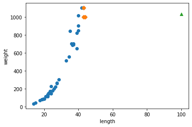
1033.3333333333333
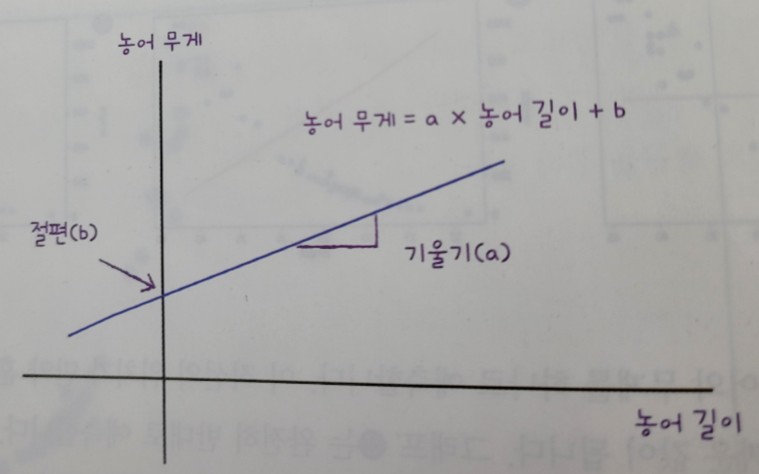
선형 회귀(linear regression)
- 비교적 간단하고 성능이 뛰어나기 때문에 맨 처음 배우는 머신러닝 알고리즘

In [6]:
from sklearn.linear_model import LinearRegression
lr = LinearRegression()

## 선형 회귀 모델 훈련
lr.fit(train_input, train_target)

## 50Cm 농어에 대해 예측
print(lr.predict([[50]]))
[1241.83860323]
하나의 직선을 그리면,
In [8]:
print('a=',lr.coef_, 'b=',lr.intercept_)
a= [39.01714496] b= -709.0186449535474
Graph y = ax + b: 농어 길이가 15Cm - 50Cm까지
- (15, 1539-709) ~ (50, 5039-709)
In [15]:
## 훈련 세트의 산점도 그리기
plt.scatter(train_input, train_target)

## 15Cm - 50Cm까지 1차 방정식 그래프 그리기
plt.plot([15, 50], [15*lr.coef_+lr.intercept_, 50*lr.coef_+lr.intercept_])

## 50Cm 농어 데이터
plt.scatter(50, 1241.8, marker='^')
plt.xlabel('perch_length')
plt.ylabel('perch_weight')
plt.show
Out[15]:
<function matplotlib.pyplot.show(close=None, block=None)>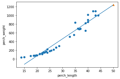
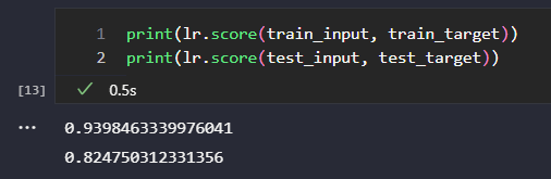
훈련세트와 테스트세트의 R^2 점수 확인.
- 훈련세트의 범위를 벗어난 농어의 무게도 예측 가능.
In [13]:
print(lr.score(train_input, train_target))
print(lr.score(test_input, test_target))
0.9398463339976041
0.824750312331356
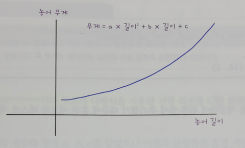
다항 회귀(polynomial Regression)
- 농어의 무게가 0g 이하로 내려갈 경우가 발생
In [16]:
## 훈련 세트의 산점도 그리기
plt.scatter(train_input, train_target)

## 1Cm - 50Cm까지 1차 방정식 그래프 그리기
plt.plot([1, 50], [1*lr.coef_+lr.intercept_, 50*lr.coef_+lr.intercept_])

## 50Cm 농어 데이터
plt.scatter(50, 1241.8, marker='^')
plt.xlabel('perch_length')
plt.ylabel('perch_weight')
plt.show
Out[16]:
<function matplotlib.pyplot.show(close=None, block=None)>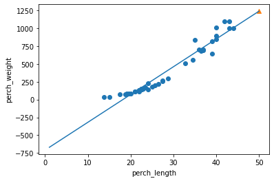
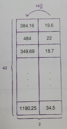
numpy의 column_stack()으로 길이, 길이^2 을 붙여서 생성 가능
- numpy의 브로드캐스팅 적용하여 train_input ** 2 식이 가능
In [22]:
## 브로드캐스팅 및 np.column_stack()으로 계산하고 합치기
train_poly = np.column_stack((train_input ** 2, train_input))
test_poly = np.column_stack((test_input ** 2, test_input))

print('2차원 2개 배열:', train_poly.shape, test_poly.shape)
print('2차원 1개 배열:', train_input.shape)
2차원 2개 배열: (42, 2) (14, 2)
2차원 1개 배열: (42, 1)
In [27]:
## polynomial regression 훈련
lr.fit(train_poly, train_target)

## 50Cm인 농어의 길이 예측하기
print('50Cm with polynomial:', lr.predict([[50**2, 50]]))

print(lr.coef_, lr.intercept_)
50Cm with polynomial: [1573.98423528]
[  1.01433211 -21.55792498] 116.0502107827827
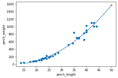
Graph y = ax^2 + bx + c: 농어의 길이가 15Cm부터 50Cm까지
In [32]:
## 구간별 곡선을 그리기 위해서 15 - 50까지 정수배열 생성
list_len = np.arange(15, 51)

## 훈련 세트의 산점도를 그리기
plt.scatter(train_input, train_target)

## 15에서 50까지 2차 곡선을 그리기
plt.plot(list_len, 1.01*list_len**2 -21.56*list_len + 116.05)

## 50Cm 농어 데이터 포함
plt.scatter(50, 1573, marker='^')
plt.xlabel('perch_length')
plt.ylabel('perch_weight')
plt.show()
In [33]:
## 훈련세트와 테스트 세트 R^2 점수 확인
print(lr.score(train_poly, train_target))
print(lr.score(test_poly, test_target))
0.9706807451768623
0.9775935108325122
선형일 경우와 비교했을 경우, score점수가 올라감.
'책[이해 및 학습]' 카테고리의 다른 글
| 2. [혼자 공부하는 머신러닝/딥러닝] 인공 신경망(ANN) (0) | 2024.03.09 |
|---|---|
| 1. [혼자 공부하는 머신러닝/딥러닝] 로지스틱 회귀로 분석 (0) | 2024.03.09 |
| 07_과대적합(overfitting) vs 과소적합(underfitting) (0) | 2023.01.03 |
| 6. [혼자 공부하는 머신러닝] 회귀(Regression): k-최근접 이웃회귀 (0) | 2023.01.03 |
| 3. [혼자 공부하는 머신러닝/딥러닝] 심층 신경망(DNN) (0) | 2022.07.22 |


