Target
1) 데이터의 전처리의 필요성에 대해서 알아보자.
2) sklearn의 고급 함수 사용 / Python 리스트보다 효율적인 넘파일 배열사용(Low level)
데이터를 준비해 보자.
## Raw data: 도미와 빙어.
bream_length = [25.4, 26.3, 26.5, 29.0, 29.0, 29.7, 29.7, 30.0, 30.0, 30.7, 31.0, 31.0, 31.5, 32.0, 32.0, 32.0, 33.0, 33.0, 33.5, 33.5, 34.0, 34.0, 34.5, 35.0, 35.0, 35.0, 35.0, 36.0, 36.0, 37.0, 38.5, 38.5, 39.5, 41.0, 41.0]
bream_weight = [242.0, 290.0, 340.0, 363.0, 430.0, 450.0, 500.0, 390.0, 450.0, 500.0, 475.0, 500.0, 500.0, 340.0, 600.0, 600.0, 700.0, 700.0, 610.0, 650.0, 575.0, 685.0, 620.0, 680.0, 700.0, 725.0, 720.0, 714.0, 850.0, 1000.0, 920.0, 955.0, 925.0, 975.0, 950.0]
smelt_length = [9.8, 10.5, 10.6, 11.0, 11.2, 11.3, 11.8, 11.8, 12.0, 12.2, 12.4, 13.0, 14.3, 15.0]
smelt_weight = [6.7, 7.5, 7.0, 9.7, 9.8, 8.7, 10.0, 9.9, 9.8, 12.2, 13.4, 12.2, 19.7, 19.9]
## 도미데이터와 빙어데이터 합치기
fish_length = bream_length + smelt_length
fish_weight = bream_weight + smelt_weight
print(fish_length)
print(fish_weight)[25.4, 26.3, 26.5, 29.0, 29.0, 29.7, 29.7, 30.0, 30.0, 30.7, 31.0, 31.0, 31.5, 32.0, 32.0, 32.0, 33.0, 33.0, 33.5, 33.5, 34.0, 34.0, 34.5, 35.0, 35.0, 35.0, 35.0, 36.0, 36.0, 37.0, 38.5, 38.5, 39.5, 41.0, 41.0, 9.8, 10.5, 10.6, 11.0, 11.2, 11.3, 11.8, 11.8, 12.0, 12.2, 12.4, 13.0, 14.3, 15.0]
[242.0, 290.0, 340.0, 363.0, 430.0, 450.0, 500.0, 390.0, 450.0, 500.0, 475.0, 500.0, 500.0, 340.0, 600.0, 600.0, 700.0, 700.0, 610.0, 650.0, 575.0, 685.0, 620.0, 680.0, 700.0, 725.0, 720.0, 714.0, 850.0, 1000.0, 920.0, 955.0, 925.0, 975.0, 950.0, 6.7, 7.5, 7.0, 9.7, 9.8, 8.7, 10.0, 9.9, 9.8, 12.2, 13.4, 12.2, 19.7, 19.9]
1) 기존 code
fish_data = [[l, w] for l, w in zip(length, weight)]
fish_target = [1] * 35 + [0] * 14
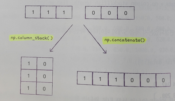
- numpy의 column_stack() 함수는 전달받은 리스트를 일렬로 세운 다음 차례대로 나란히 연결.
- numpy의 np.ones() / np.zeros()로 Target데이터 생성 가능.
- 데이터가 클수록, 파이썬 리스트는 비효율적이므로 넘파이 배열사용(low level 언어)을 추천.
- 2개 리스트 & 배열을 세로로 1개씩 붙이면 ==> np.column_stack
- 2개 리스트 & 배열을 가로로 쭉 붙이면 ==> np.concatenate
기존 code보다는 보다 효율적인 넘파이 사용하여 데이터 배열 준비.
import numpy as np
fish_data = np.column_stack((fish_length, fish_weight))
fish_target = np.concatenate((np.ones(35), np.zeros(14)))
print(fish_data)
print(fish_target)
<결과물>
[[  25.4  242. ]
 [  26.3  290. ]
 [  26.5  340. ]
 [  29.   363. ]
 [  29.   430. ]
 [  29.7  450. ]
 [  29.7  500. ]
 [  30.   390. ]
 [  30.   450. ]
 [  30.7  500. ]
 [  31.   475. ]
 [  31.   500. ]
 [  31.5  500. ]
 [  32.   340. ]
 [  32.   600. ]
 [  32.   600. ]
 [  33.   700. ]
 [  33.   700. ]
 [  33.5  610. ]
 [  33.5  650. ]
 [  34.   575. ]
 [  34.   685. ]
 [  34.5  620. ]
 [  35.   680. ]
 [  35.   700. ]
 [  35.   725. ]
 [  35.   720. ]
 [  36.   714. ]
 [  36.   850. ]
 [  37.  1000. ]
 [  38.5  920. ]
 [  38.5  955. ]
 [  39.5  925. ]
 [  41.   975. ]
 [  41.   950. ]
 [   9.8    6.7]
 [  10.5    7.5]
 [  10.6    7. ]
 [  11.     9.7]
 [  11.2    9.8]
 [  11.3    8.7]
 [  11.8   10. ]
 [  11.8    9.9]
 [  12.     9.8]
 [  12.2   12.2]
 [  12.4   13.4]
 [  13.    12.2]
 [  14.3   19.7]
 [  15.    19.9]]
[1. 1. 1. 1. 1. 1. 1. 1. 1. 1. 1. 1. 1. 1. 1. 1. 1. 1. 1. 1. 1. 1. 1. 1.
 1. 1. 1. 1. 1. 1. 1. 1. 1. 1. 1. 0. 0. 0. 0. 0. 0. 0. 0. 0. 0. 0. 0. 0.
 0.]
sklearn.model_selection / train_test_split()로 전달되는 리스트나 배열 나누기.
- train set / test set 구분
- 기존 Code
[np.random.seed(42)
index = np.arange(49)
np.random.shuffle(index)]

from sklearn.model_selection import train_test_split        # 리스트나 배열을 비율에 따라 나누기.
train_input, test_input, train_target, test_target = train_test_split(fish_data, fish_target, random_state=42)
print('train_input 형태:', train_input.shape, 'test_input 형태:', test_input.shape)
print('train_target 형태:', train_target.shape, 'test_target 형태:', test_target.shape)
print(test_target)
list_test_target = list(test_target)
print(list_test_target.count(1), list_test_target.count(0))
print()
<결과물>
train_input 형태: (36, 2) test_input 형태: (13, 2)
train_target 형태: (36,) test_target 형태: (13,)
[1. 0. 0. 0. 1. 1. 1. 1. 1. 1. 1. 1. 1.]
10 3
- split 함수 & random_state로 무작위로 데이터를 나누었을 때, 샘플이 골고루 섞이지 않는다
(샘플링 편향이 또 발생). ==> 해결: stratify
train_input, test_input, train_target, test_target = train_test_split(fish_data, fish_target, stratify=fish_target, random_state=42)
print(test_target)
list_test_target_stratify = list(test_target)
print(list_test_target_stratify.count(1), list_test_target_stratify.count(0))
[0. 0. 1. 0. 1. 0. 1. 1. 1. 1. 1. 1. 1.]
9 4
## K-최근접 이웃(훈련 데이터를 저장하는 것으로만 훈련 진행)
from sklearn.neighbors import KNeighborsClassifier          # 어떤 규칙을 찾기보다는, 전체 데이터를 메모리에 가지고 있음.
kn = KNeighborsClassifier()
kn.fit(train_input, train_target)
print('test score:', kn.score(test_input, test_target))
print("25, 150 인 경우 구분:", kn.predict([[25, 150]]))
test score: 1.0
25, 150 인 경우 구분: [0.]
## 수상한 도미 한마리 그리기
import matplotlib.pyplot as plt                             # matplotlib의 plot함수를 plt로 줄여서 사용.
plt.scatter(train_input[:, 0], train_input[:, 1])
plt.scatter(test_input[:, 0], test_input[:, 1])
plt.scatter(25, 150, marker='^')
plt.show()
investigation for K-최근접 이웃 데이터(이웃데이터 5개 참조)
plt.scatter(train_input[:, 0], train_input[:, 1])
plt.scatter(test_input[:, 0], test_input[:, 1])
plt.scatter(25, 150, marker='^')

distances, indexes = kn.kneighbors([[25, 150]])
plt.scatter(train_input[indexes, 0], train_input[indexes, 1], marker='D')
plt.title('investigation')
plt.xlabel('length')
plt.ylabel('weight')
plt.show()
print("5개 sample --> length & weight:", train_input[indexes])
print("5개 sample --> 도미 & 빙어", train_target[indexes])
print("5개 sample <-> [25, 150] 거리", distances)
5개 sample --> length & weight: [[[ 25.4 242. ]
[ 15. 19.9]
[ 14.3 19.7]
[ 13. 12.2]
[ 12.2 12.2]]]
5개 sample --> 도미 & 빙어 [[1. 0. 0. 0. 0.]]
5개 sample <-> [25, 150] 거리 [[ 92.00086956 130.48375378 130.73859415 138.32150953 138.39320793]]

Re-scaling ==> X and Y 축을 같게 설정.
plt.scatter(train_input[:, 0], train_input[:, 1])
plt.scatter(25, 150, marker='^')
plt.scatter(train_input[indexes, 0], train_input[indexes, 1], marker='D')
plt.xlim((0, 1000))
plt.title("Re-scale")
plt.xlabel('length')
plt.ylabel('weight')
plt.show()
- X축 범위가 좁고, y축은 넓어서 --> y축으로 조금만 멀어져도 거리가 아주 큰 값으로 계산.
- 이를 두 특성의 스케일(scale)이 다르다고 말한다.
- 특성값을 일정한 기준으로 맞춰주는 작업 ==> 데이터 전처리(Data preprocessing)
- 가장 널리 사용하는 전처리 방법 중 하나 ==> 표준점수(standard score & z점수)
- 표준점수는 각 특성값이 0에서 표준편차의 몇 배만큼 떨어져 있는지 확인.
mean = np.mean(train_input, axis=0)             # 2차원 list형태에서 axis = 0은 세로를 의미 / axis = 1은 가로를 의미
std = np.std(train_input, axis=0)
print()
print("평균", mean, "표준편차", std)
평균 [ 27.29722222 454.09722222] 표준편차 [ 9.98244253 323.29893931]

## train_scaled 구하고 다시 훈련시키기
## 브로드캐스팅은 넘파이 배열 사이에서 발생
train_scaled = (train_input - mean) / std
kn.fit(train_scaled, train_target)


plt.scatter(train_scaled[:, 0], train_scaled[:, 1])
plt.scatter(25, 150, marker='^')
plt.title('[25, 150] not scaled')
plt.xlabel('length')
plt.ylabel('weight')
plt.show()
## [25, 150] 역시 훈련세트의 mean / std를 반영해야 함.
new = ([25, 150] - mean) / std
distances, indexes = kn.kneighbors([new])

plt.scatter(train_scaled[:,0], train_scaled[:,1])
plt.scatter(new[0], new[1], marker='^')
plt.scatter(train_scaled[indexes, 0], train_scaled[indexes, 1], marker='D')
plt.title('final plot')
plt.xlabel('length')
plt.ylabel('weight')
plt.show()


## Test set 역시, 훈련세트의 mean & std 반영해야 함.
test_scaled = (test_input - mean) / std
print("평가: ", kn.score(test_scaled, test_target))
print("도미 vs 빙어 -->", kn.predict([new]))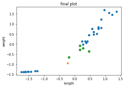
평가:  1.0
도미 vs 빙어 --> [1.]'Machine Learning with Python' 카테고리의 다른 글
| 6_하이퍼파라미터 튜닝 (0) | 2022.07.06 |
|---|---|
| 5_트리의 앙상블(Ensemble Learning) (0) | 2022.07.05 |
| 1_첫번째 머신러닝: KNeighborsClassifier (0) | 2022.04.15 |
| [간단정리: Machine Learning] - cross validation편- (0) | 2021.10.27 |
| 구글 코랩 / 주피터 노트북 사용기 (0) | 2021.09.21 |


